Generating random variables with given variance-covariance matrix can be useful for many purposes. For example it is useful for generating random intercepts and slopes with given correlations when simulating a multilevel, or mixed-effects, model (e.g. see here). This can be achieved efficiently with the Choleski factorization. In linear algebra the factorization or decomposition of a matrix is the factorization of a matrix into a product of matrices. More specifically, the Choleski factorization is a decomposition of a positive-defined, symmetric1 matrix into a product of a triangular matrix and its conjugate transpose; in other words is a method to find the square root of a matrix. The square root of a matrix \(C\) is another matrix \(L\) such that \({L^T}L = C\).2
Suppose you want to create 2 variables, having a Gaussian distribution, and a positive correlation, say \(0.7\). The first step is to define the correlation matrix \[C = \left( {\begin{array}{*{20}{c}} 1&{0.7}\\ {0.7}&1 \end{array}} \right)\] Elements in the diagonal can be understood as the correlation of each variable with itself, and therefore are 1, while elements outside the diagonal indicate the desired correlation. In \(\textsf{R}\)
C <- matrix(c(1,0.7,0.7,1),2,2)Next one can use the chol() function to compute the Cholesky factor. (The function provides the upper triangular square root of \(C\)).
L <- chol(C)If you multiply the matrix \(L\) with itself you get back the original correlation matrix (\(\textsf{R}\) output below).
t(L) %*% L
     [,1] [,2]
[1,]  1.0  0.7
[2,]  0.7  1.0
Then we need another matrix with the desired standard deviation in the diagonal (in this example I choose 1 and 2)
tau <- diag(c(1,2))Multiply that matrix with the lower triangular square root of the correlation matrix (can be obtained by taking the transpose of \(L\))
Lambda <- tau %*% t(L)Now we can generate values for 2 independent random variables \(z\sim\cal N\left( {0,1} \right)\)
Z <- rbind(rnorm(1e4),rnorm(1e4))Finally, to introduce the correlations , multiply them with the Lambda obtained above
X <- Lambda %*% ZNow plot the results
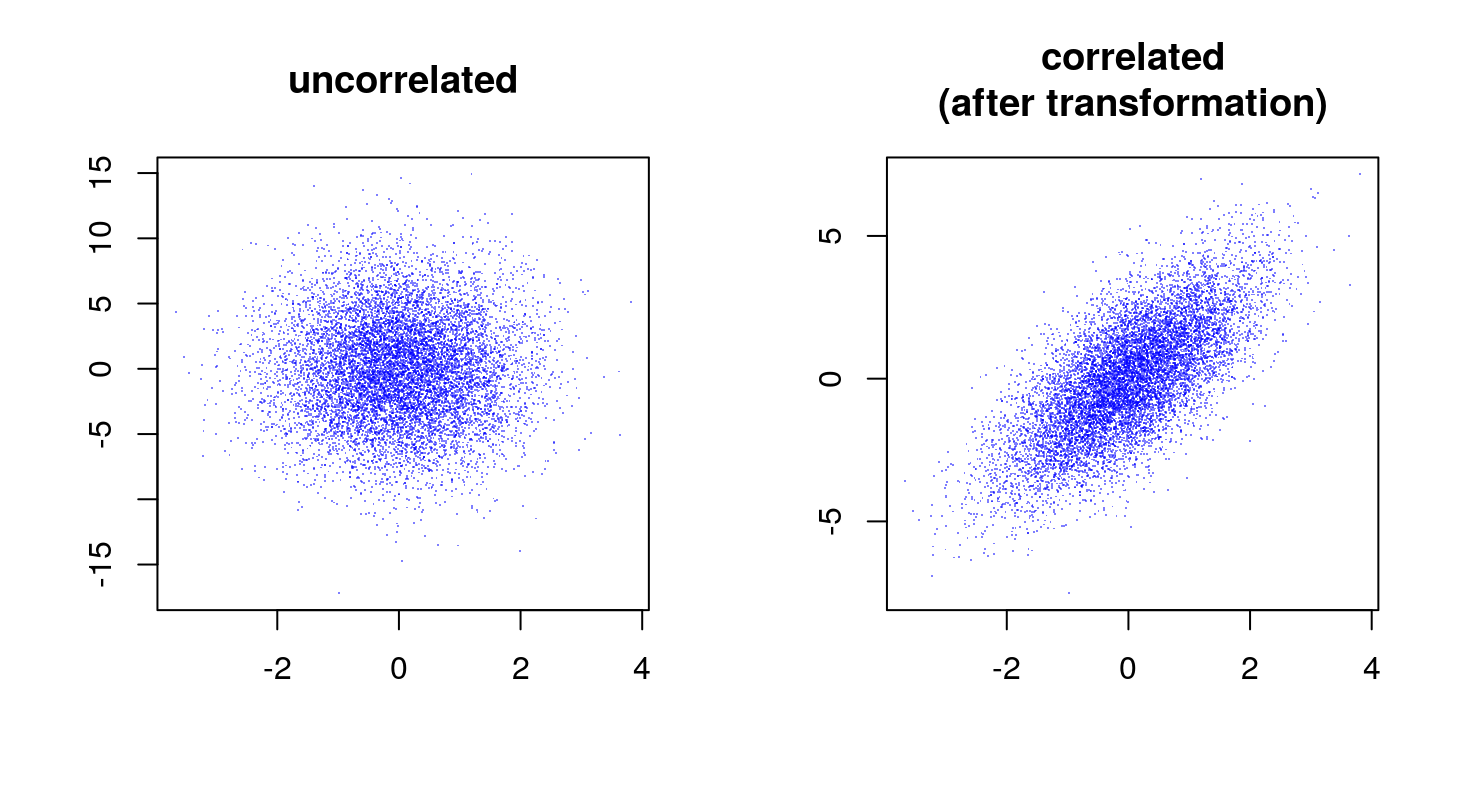 We can verify that the correlation as estimated from the sample corresponds (or is close enough) to the generative value.
# correlation in the generated sample
cor(X[1,],X[2,])
[1] 0.7093591
Why does it work?
The covariance matrix of the initial, uncorrelated sample is \(\mathbb{E} \left( Z Z^T \right) = I\), that is the identity matrix, since they have zero mean and unit variance \(z\sim\cal N\left( {0,1} \right)\)3.
Let’s suppose that the desired covariance matrix is \(\Sigma\); since it is symmetric and positive defined it is possible to obtain the Cholesky factorization \(L{L^T} = \Sigma\).
If we then compute a new random vector as \(X=LZ\), we have that its covariance matrix is \[ \begin{align} \mathbb{E} \left(XX^T\right) &= \mathbb{E} \left((LZ)(LZ)^T \right) \\ &= \mathbb{E} \left(LZ Z^T L^T\right) \\ &= L \mathbb{E} \left(ZZ^T \right) L^T \\ &= LIL^T = LL^T = \Sigma \\ \end{align} \] Therefore the new random vector \(X\) has the covariance matrix \(\Sigma\).
The third step is justified because the expected value is a linear operator, therefore \(\mathbb{E}(cX) = c\mathbb{E}(X)\). Also \((AB)^T = B^T A^T\), note that the order of the factor reverses.
Actually Choleski factorization can be obtained from all Hermitian matrices. Hermitian matrices are a complex extension of real symmetric matrices. A symmetric matrices is one that it is equal to its transpose, which implies that its entries are symmetric with respect to the diagonal. In a Hermitian matrix, symmetric entries with respect to the diagonal are complex conjugates, i.e. they have the same real part, and an imaginary part with equal magnitude but opposite in sign. For example, the complex conjugate of \(x+iy\) is \(x-iy\) (or, equivalently, \(re^{i\theta}\) and \(re^{-i\theta}\)). Real symmetric matrices can be considered a special case of Hermitian matrices where the imaginary component \(y\) (or \(\theta\)) is \(0\).↩
Note that I am using the convention of \(\textsf{R}\) software, where the function
chol(), which compute the factorization, returns the upper triangular factor of the Choleski decomposition. I think that is more commonly assumed that the Choleski decomposition returns the lower triangular factor \(L\), in which case \(L{L^T} = C\).↩More generally the variance-covariance matrix is \(\Sigma = \mathbb{E}\left( {X{X^T}} \right) - \mathbb{E}\left( X \right) \mathbb{E}\left(X \right)^T\). \(\mathbb{E}\) indicates the expected value.↩