In the study of human perception we often need to measure how sensitive is an observer to a stimulus variation, and how her/his sensitivity changes due to changes in the context or experimental manipulations. In many applications this can be done by estimating the slope of the psychometric function1, a parameter that relates to the precision with which the observer can make judgements about the stimulus. A psychometric function is generally characterized by 2-3 parameters: the slope, the threshold (or criterion), and an optional lapse parameter, which indicate the rate at which attention lapses (i.e. stimulus-independent errors) occur.
As an example, consider the situation where an observer is asked to judge whether a signal (can be anything, from the orientation angle of a line on a screen, or the pitch of a tone, to the speed of a car or the approximate number of people in a crowd, etc.) is above or below a given reference value, call it zero. The experimenter presents the observers with many signals of different intensities, and the observer is asked to respond by making a binary choice (larger/smaller than the reference), under two different contextual conditions (before/after having a pint, with different headphones, etc.). These two conditions are expected to results in different sensitivity, and the experimenter is interested in estimating as precisely as possible the difference in sensitivity2. The psychometric function for one observer in the two conditions might look like this (figure below).
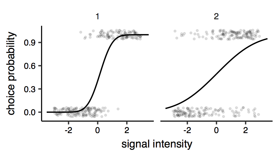
Psychometric functions. Each points is a response (0 or 1 ; some vertical jitter is added for clarity), and the lines represent the fitted psychometric model (here a cumulative Gaussian psychometric function). The two facets of the plots represent the two different conditions. It can be seen that the precision seems to be different across conditions: judgements made under condition ‘2’ are more variable, indicating reduced sensitivity.
Our focus is on the psychometric slope, and we are not really interested in measuring the lapse rate; however it is still important to take lapses into account: it has been shown that not accounting for lapses can have a large influence on the estimates of the slope (Wichmann and Hill 2001).
The problem with lapses
Different observer may lapse at quite different rates, and for some of them the lapse rate is probably so small that can be considered negligible. Also, we usually don’t have hypothesis about lapses, and about whether they should or should not vary across conditions. We can base our analysis on different assumptions about when the observers may have attention lapses:
- they may never lapse (or they do so with a small, negligible frequency);
- they may lapse at a fairly large rate, but the rate is assumed constant across conditions (reasonable, especially if conditions are randomly interleaved);
- they may lapse with variable rate across conditions.
These assumptions will lead to three different psychometric models. The number can increase if we consider also different functional forms of the relationship between stimulus and choice; here for simplicity I will consider only psychometric models based on the cumulative Gaussian function (equivalent to a probit analysis), \(\Phi (\frac{x-\mu}{\sigma}) = \frac{1}{2}\left[ {1 + {\rm{erf}}\left( {\frac{{x - \mu }}{{\sigma \sqrt 2 }}} \right)} \right]\), where the mean \(\mu\) woud correspond to the threshold parameter, \(\sigma\) to the slope, and \(x\) is the stimulus intensity. In our case the first assumption (zero lapses) would lead to the simplest psychometric model \[ \Psi (x, \mu_i, \sigma_i)= \Phi (\frac{x-\mu_i}{\sigma_i}) \] where the subscript \(i\) indicates that the values of both mean \(\mu_i\) and slope \(\sigma_i\) are specific to the condition \(i\). The second assumption (fixed lapse rate) could correspond to the model \[ \Psi (x, \mu_i, \sigma_i, \lambda)= \lambda + (1-2\lambda) \Phi (\frac{x-\mu_i}{\sigma_i}) \] where the parameter \(\lambda\) correspond to the probability of the observer making a random error. Note that this is assumed to be fixed with respect to the condition (no subscript). Finally the last assumption (variable lapse rate) would suggests the model \[ \Psi (x, \mu_i, \sigma_i, \lambda_i)= \lambda_i + (1-2\lambda_i) \Phi (\frac{x-\mu_i}{\sigma_i}) \] where all the parameters are allowed to vary between conditions.
We have thus three different models, but we haven’t any prior information to decide which model is more likely to be correct in our case. Also, we acknowledge the fact that there are individual differences and each observer in our sample may conform to one of the three assumptions with equal probability. Hence, ideally, we would like to find a way to deal with lapses - and find the best estimates of the slope values \(\sigma_i\) without committing to one of the three models.
Multi-model inference
One possible solution to this problem is provided by a multi-model, or model averaging, approach (Burnham and Anderson 2002). This requires calculating the AIC (Akaike Information Criterion)3 for each model and subjects, and then combine the estimates according to the Akaike weights of each model. To compute the Akaike weights one typically proceed by first transforming them into differences with respect to the AIC of the best candidate model (i.e. the one with lower AIC) \[ {\Delta _m} = {\rm{AI}}{{\rm{C}}_m} - \min {\rm{AIC}} \] From the differences in AIC, we can obtain an estimate of the relative likelihood of the model \(m\) given the data \[ \mathcal{L} \left( {m|{\rm{data}}} \right) \propto \exp \left( { - \frac{1}{2}{\Delta _m}} \right) \] Then, to obtain the Akaike weight \(w_m\) of the model \(m\), the relative likelihoods are normalized (divided by their sum) \[ {w_m} = \frac{{\exp \left( { - \frac{1}{2}{\Delta _m}} \right)}}{{\mathop \sum \limits_{k = 1}^K \exp \left( { - \frac{1}{2}{\Delta _k}} \right)}} \] Finally, one can compute the model-averaged estimate of the parameter4, \(\hat {\bar \sigma}\), by combining the estimate of each model according to their Akaike weight \[ \hat {\bar \sigma} = \sum\limits_{k = 1}^K {{w_k}\hat \sigma_k } \]
Simulation results
Model averaging seems a sensitive approach to deal with the uncertainty about which form of the model is best suited to our data. To see whether it is worth doing the extra work of fitting 3 models instead of just one, I run a simulation, where I repeatedly fit and compare the estimates of the three models, with the model-averaged estimate, for different values of sample sizes. In all the simulations, each observer is generated by randomly drawing parameters from a Gaussian distribution which summarize the distribution of the parameters in the population. Hence, I know the true difference in sensitivity in the population, and by simulating and fitting the models I can test which estimating procedure is more efficient. In statistics a procedure or an estimator is said to be more efficient than another one when it provides a better estimate with the same number or fewer observations. The notion of “better” clearly relies on the choice of a cost function, which for example can be the mean squared error (it is here).
Additionally, in my simulations each simulated observer could, with equal probability \(\frac{1}{3}\), either never lapse, lapse with a constant rate across conditions, or lapse at a higher rate in the more difficult condition (condition ‘2’ where the judgements are less precise). The lapse rates were draw uniformly from the interval [0.01, 0.1], and could get as high as 0.15 in condition ‘2’. Each simulated observer ran 250 trials per condition (similar to the figure at the top of this page). I simulated dataset from \(n=5\) to \(n=50\), using 100 iterations for each sample size (only 85 in the case of \(n=50\) because the simulation was taking too long and I needed my laptop for other stuff). For simplicity I assumed that the different parameters were not correlated across observers5. I also had my simulated observer using the same criterion across the two conditions, although this may not necessarily be true. The quantity of interest here is the difference in slope between the two condition, that is \(\sigma_2 - \sigma_1\).
First, I examined the mean squared error of each of the models’ estimates, and of the model-averaged estimate. This is the average squared difference between the estimate and the true value.
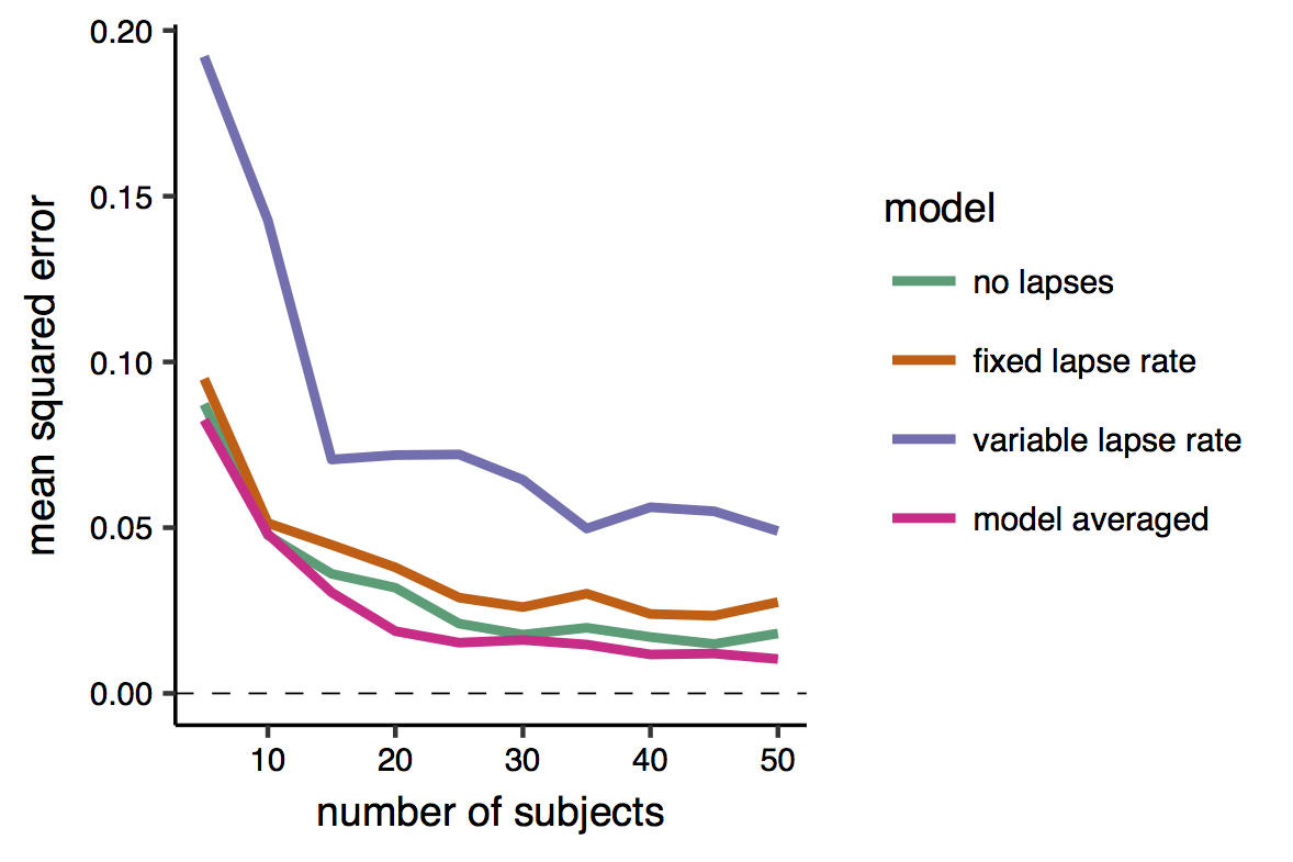 The results shows (unless my color blindness fooled me) that the model-averaged estimate attains always the smaller error. Note also that the error tend to decrease exponentially with the sample size. Interestingly, the worst model seems to be the one that allow for the lapses to vary across conditions. This may be because the change in the lapse rate across condition was - when present - relatively small, but also because this model has a larger number of parameters, and thus produces more variable estimates (that is with higher standard errors) than smaller model. Indeed, given that I know the ‘true’ value of the parameres in this simulation settings, I can divide the error into the two subcomponents of variance and bias (see this page for a nice introduction to the bias-variance tradeoff). The bias is the difference between the expected estimate (averaged over many repetitions/iterations) of the same model and the true quantity that we want to estimate. The variance is simply the variability of the model estimates, i.e. how much they oscillate around the expected estimate.
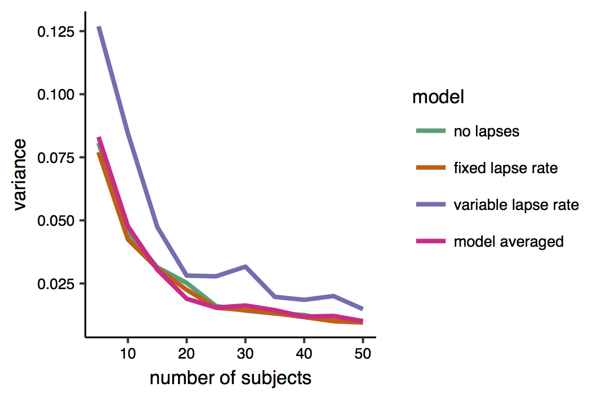
Here is a plot of the variance. Indeed it can be seen that the variable-lapse model, which has more parameters, is the one that produces more variable estimates. There is however little difference between the other two models’ and the multi-model estimates
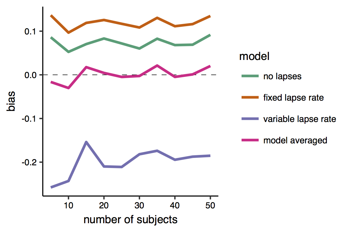
And here is the bias. This is very satisfactory, as it shows that while all individual models produced biased estimates, the bias of the model-averaged estimates is zero, or very close to zero.
 In sum, by averaging models of different levels of complexity according to their relative likelihood, I was able to simultaneously minimize the variance and decrease the bias of my estimates, and achieve a greater efficiency. Model averaging seems to be the ideal procedure in this specific settings where the observer would belong to one of the three categories (i.e., she/he would conform to one of the three assumptions) with equal probability. However I think (although I haven’t checked) that it would perform well even in cases where a single “type” of observers is largely predominant over the other.
Code
The (clumsy written) code for the simulations is shown below:
# This load some handy functions that are required below
library(RCurl)
script <- getURL("https://raw.githubusercontent.com/mattelisi/miscR/master/miscFunctions.R", ssl.verifypeer = FALSE)
eval(parse(text = script))

set.seed(1)

# sim parameters
n_sim <- 100
sample_sizes <- seq(5, 100, 5)

# parameters
R <- 3 # range of signal levels (-R, R)
n_trial <- 500
mu_par <- c(0, 0.25) # population (mean, std.)
sigma_par <- c(1, 0.25)
sigmaDiff_par <- c(1, 0.5)
lapse_range <- c(0.01, 0.1)

# start
res <- {}
for(n_subjects in sample_sizes){
for(iteration in 1:n_sim){

    # make dataset
    d <- {}
    for(i in 1:n_subjects){
        d_ <- data.frame(x=runif(n_trial)*2*R-R,
                    condition=as.factor(rep(1:2,n_trial/2)),
                    id=i, r=NA)

        r_i <- runif(1) # draw observer type (wrt lapses)

        if(r_i<1/3){
            # no lapses
            par1 <- c(rnorm(1,mu_par[1],mu_par[2]),
                abs(rnorm(1,sigma_par[1],sigma_par[2])),
                0)
            par2 <- c(par1[1],
                par1[2]+abs(rnorm(1,sigmaDiff_par[1],sigmaDiff_par[2])),
                0)

        }else if(r_i>=1/3 & r_i<2/3){
            # fixed lapses
            l_i <- runif(1)*diff(lapse_range) + lapse_range[1]
            par1 <- c(rnorm(1,mu_par[1],mu_par[2]),
                abs(rnorm(1,sigma_par[1],sigma_par[2])),
                l_i)
            par2 <- c(par1[1],
                par1[2]+abs(rnorm(1,sigmaDiff_par[1],sigmaDiff_par[2])),
                l_i)

        }else{
            # varying lapses
            l_i_1 <- runif(1)*diff(lapse_range) + lapse_range[1]
            l_i_2 <- l_i_1 + (runif(1)*diff(lapse_range) + lapse_range[1])/2
            par1 <- c(rnorm(1,mu_par[1],mu_par[2]),
                abs(rnorm(1,sigma_par[1],sigma_par[2])),
                l_i_1)
            par2 <- c(par1[1],
                par1[2]+abs(rnorm(1,sigmaDiff_par[1],sigmaDiff_par[2])),
                l_i_2)
        }

        ## simulate observer
        for(i in 1:sum(d_$condition=="1")){
            d_$r[d_$condition=="1"][i] <- rbinom(1,1,
                psy_3par(d_$x[d_$condition=="1"][i],par1[1],par1[2],par1[3]))
        }
        for(i in 1:sum(d_$condition=="2")){
            d_$r[d_$condition=="2"][i] <- rbinom(1,1,
                psy_3par(d_$x[d_$condition=="2"][i],par2[1],par2[2],par2[3]))
        }
        d <- rbind(d,d_)
    }


    ## model fitting

    # lapse assumed to be 0
    fit0 <- {}
    for(j in unique(d$id)){
        m0 <- glm(r~x*condition, family=binomial(probit),d[d$id==j,])
        sigma_1 <- 1/coef(m0)[2]
        sigma_2 <- 1/(coef(m0)[2] + coef(m0)[4])
        fit0 <- rbind(fit0, data.frame(id=j, sigma_1, sigma_2,
                loglik=logLik(m0), aic=AIC(m0), model="zero_lapse") )
    }

    # fix lapse rate
    start_p <- c(rep(c(0,1),2), 0)
    l_b <- c(rep(c(-5, 0.05),2), 0)
    u_b <- c(rep(c(5, 20), 2), 0.5)
    fit1 <- {}

    for(j in unique(d$id)){
        ftm <- optimx::optimx(par = start_p, lnorm_3par_multi ,
                d=d[d$id==j,],  method="bobyqa",
                lower =l_b, upper =u_b)

        negloglik <- ftm$value
        aic <- 2*5 + 2*negloglik
        # fitted parameters are the first n numbers of optimx output
        sigma_1<-unlist(ftm [1,2])
        sigma_2<-unlist(ftm [1,4])
        fit1 <- rbind(fit1, data.frame(id=j, sigma_1, sigma_2,
                loglik=-negloglik, aic, model="fix_lapse")  )
    }


    # varying lapse rate
    start_p <- c(0,1, 0)
    l_b <- c(-5, 0.05, 0)
    u_b <- c(5, 20, 0.5)
    fit2 <- {}
    for(j in unique(d$id)){
        # fit condition 1
        ftm <- optimx::optimx(par = start_p, lnorm_3par ,
                d=d[d$id==j & d$condition=="1",],
                method="bobyqa", lower =l_b, upper =u_b)
        negloglik_1 <- ftm$value; sigma_1 <- unlist(ftm [1,2])
        # fit condition 2
        ftm <- optimx::optimx(par = start_p, lnorm_3par ,
                d=d[d$id==j & d$condition=="2",],
                method="bobyqa", lower =l_b, upper =u_b)
        negloglik_2 <- ftm$value; sigma_2 <- unlist(ftm [1,2])

        aic <- 2*6 + 2*(negloglik_1 + negloglik_2)
        fit2 <- rbind(fit2, data.frame(id=j, sigma_1, sigma_2,
                loglik=-negloglik_1-negloglik_2, aic, model="var_lapse"))
    }

    # compute estimates of the change in slope
    effect_0 <- mean((fit0$sigma_2-fit0$sigma_1))
    effect_1 <- mean((fit1$sigma_2-fit1$sigma_1))
    effect_2 <- mean((fit2$sigma_2-fit2$sigma_1))

    effect_av <- {}
    for(j in unique(fit0$id)){
        dj <- rbind(fit0[fit0$id==j,], fit1[fit1$id==j,], fit2[fit2$id==j,])
        min_aic <- min(dj$aic)
        dj$delta <- dj$aic - min_aic
        den <- sum(exp(-0.5*c(dj$delta)))
        dj$w <- exp(-0.5*dj$delta) / den
        effect_av <- c(effect_av, sum((dj$sigma_2-dj$sigma_1) * dj$w))
    }
    effect_av <- mean(effect_av)

    # store results
    res <- rbind(res, data.frame(effect_0, effect_1, effect_2,
            effect_av, effect_true=sigmaDiff_par[1],
            n_subjects, n_trial, iteration))

}
}

## PLOT RESULTS
library(ggplot2)
library(reshape2)

res$err0 <- (res$effect_0 -1)^2
res$err1 <- (res$effect_1 -1)^2
res$err2 <- (res$effect_2 -1)^2
res$errav <- (res$effect_av -1)^2

# plot MSE
ares <- aggregate(cbind(err0,err1,err2,errav)~n_subjects, res, mean)
ares <- melt(ares, id.vars=c("n_subjects"))
levels(ares$variable) <- c("no lapses", "fixed lapse rate", "variable lapse rate", "model averaged")
ggplot(ares,aes(x=n_subjects, y=value, color=variable))+geom_line(size=1)+nice_theme+scale_color_brewer(palette="Dark2",name="model")+labs(x="number of subjects",y="mean squared error")+geom_hline(yintercept=0,lty=2,size=0.2)

# plot variance
ares <- aggregate(cbind(effect_0,effect_1,effect_2,effect_av)~n_subjects, res, var)
ares <- melt(ares, id.vars=c("n_subjects"))
levels(ares$variable) <- c("no lapses", "fixed lapse rate", "variable lapse rate", "model averaged")
ggplot(ares,aes(x=n_subjects, y=value, color=variable))+geom_line(size=1)+nice_theme+scale_color_brewer(palette="Dark2",name="model")+labs(x="number of subjects",y="variance")

# plot bias
ares <- aggregate(cbind(effect_0,effect_1,effect_2,effect_av)~n_subjects, res, mean)
ares <- melt(ares, id.vars=c("n_subjects"))
levels(ares$variable) <- c("no lapses", "fixed lapse rate", "variable lapse rate", "model averaged")
ares$value <- ares$value -1
ggplot(ares,aes(x=n_subjects, y=value, color=variable))+geom_hline(yintercept=0,lty=2,size=0.2)+geom_line(size=1)+nice_theme+scale_color_brewer(palette="Dark2",name="model")+labs(x="number of subjects",y="bias")
References
Burnham, Kenneth P., and David R. Anderson. 2002. Model Selection and Multimodel Inference: A Practical Information-Theoretic Approach. 2nd editio. New York, US: Springer New York. https://doi.org/10.1007/b97636.
Wichmann, F a, and N J Hill. 2001. “The psychometric function: I. Fitting, sampling, and goodness of fit.” Perception & Psychophysics 63 (8): 1293–1313. http://www.ncbi.nlm.nih.gov/pubmed/11800458.
The psychometric function is a statistical model that predicts the probabilities of the observer response (e.g. “stimulus A has a larger/smaller instensity than stimulus B”), conditional to the stimulus and the experimental condition.↩
A good experimenter should do that (estimate the size of the difference). A “bad” experimenter might just be interested in obtaining \(p<.05\). See this page, compiled by Jean-Michel Hupé, for some references and guidelines against \(p\)-hacking and the misuse of statistical tools in neuroscience.↩
The AIC of a model is computed as \({\rm{AIC}} = 2k - 2\log \left( \mathcal{L} \right)\), where \(k\) is the number of free parameters, and \(\mathcal{L}\) is the maximum value of the likelihood function of that model.↩
Here it is a parameter common to all models. See the book of Burnham & Andersen for methods to methods to deal with different situations (Burnham and Anderson 2002).↩
Such correlation when present can be modelled using a mixed-effect approach. See my tutorial on mized-effects model in the‘misc’ section of this website.↩